Intro to hypothesis testing
In this post, we walk through a toy problem to talk about the anatomy and design of a statistical test of hypothesis. We will see
- What is a p-value and how to compute it
- What are False Positive rates and why it’s important to know them well
- How to fix a conservative bias in the decisions based on the test results
- Limitations of statistical tests
Toy problem
Would you believe it if someone told you that 1 out of 10 coin tosses came up as heads? A general approach to decide is to answer “what are the odds?!”.
The simplest ways to do that include making assumptions about how the world works and then computing the likelihood of the observed reality happening in a world like that.
Let’s assume that each coin flip is equally likely to turn out heads or tails, independently of previous coin flips. In other words, the coin is unbiased.
If that is true, then the number of heads in a stream of 10 coin tosses follows a binomial distribution with parameters 10 and 1/2 and we would expect that about half (that is, 5) of the coin flips would turn out heads. Below are the probabilities of observing each possible “heads” count:
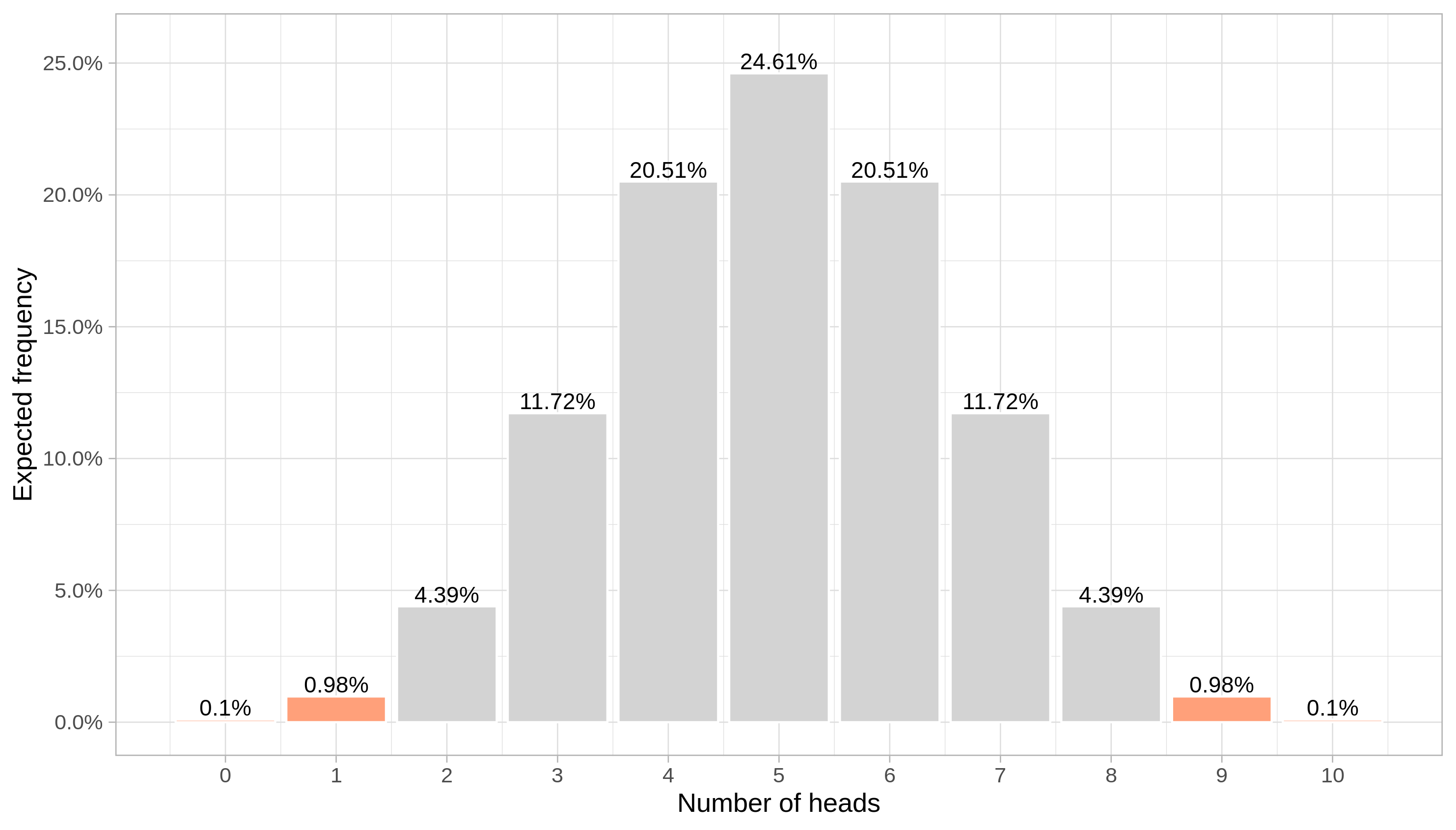
The probability of observing exactly what our friend said (1 head) would be about 0.98%.
More importantly, we can compute the tail probability of events at least as extreme as the 1 count, that is 0, 1, 9 or 10 heads count since they are all at least as far from the expected result 5 as 1. That is, they are at least as likely outcomes as 1. The result is approximately 2.15%.
You can use that number to make a call. Is 2.15% low enough for we to disbelieve that heads and tails are equally likely? Does it make the phrase “1 out of 10 were heads” sound nonsense? The decision is up to you.
You may say a number of valid things, like:
- “Since 2.15% is greater than 1%, I think the coin is indeed unbiased.”
- “That’s too unlikely! If he said the heads count was between 3 and 7 I would believe it.”
- “10 samples are not enough. I need more data to decide.”
In any case, there is a subset of outcomes for which we would reject the idea that the coin is unbiased.
Naming stuff
Well, we have pretty much done it! We have just built a statistical test. It required
- Hypothesizing a model of how the world works: The outcomes of coin flips are independent and equally likely
- Evaluating the odds of events at least as extreme as the observed reality happening if the model is true: The probability of observing heads once out of 10 coin tosses was evaluated to 0.98% and the probability of observing events like this or even more extreme (with respect to the initial hypothesis) was evaluated to 2.15%.
- Making a call based on the tail probability according to a pre-specified rule.
The assumptions we make about how the world works (“the coin is unbiased”), upon which we compute the probability of interest, compose what is usually called the null hypothesis. The tail probability (2.15%) is called the p-value.
The function of data that we use to compute the p-value (number of heads) is called the test statistic. It has a distribution under the null hypothesis (binomial, with parameters 10 and 1/2) sometimes called the null distribution. The set of outcomes who would make us doubt the null hypothesis in such a way that we reject it as a plausible description of reality (for instance, “the p-value is smaller than 1%” or “the distance of the heads count to 5 is greater than 2”) is called the critical region.
When making a decision informed by the p-value, we may be wrong in two ways:
- If we decide the coin is biased, when actually it’s not; and
- If we decide the coin is unbiased, when in fact it is biased.
The first one is called a False Positive (FP). The second one is a False Negative (FN). The null hypothesis is usually set up as the hypothetical world where
- “everything is OK”, or
- “nothing has changed”, or
- “you are healthy”, or
- “he is innocent”, or
- “there’re no differences between these groups of people”, or
- “there’s no enemy’s plane entering our borders”,
and so on. Therefore, the term “Positive” in “False Positive” refers to the detection of “something”.
Controlling the rates of FPs and FNs is a central task in the design of a statistical test. Those rates pose a trade-off to be solved by the designer:
- I don’t want to miss anything! Being too afraid of failing to catch up any deviations from the null hypothesis leads to setting too small FN rates. That may cause in turn an increase of FPs since we may shout out “I saw something!!!” for almost anything.
- I hate interruptions! In the context of quality control of industrial products, we may want to avoid stopping the machines unless something really critical is detected, and then very small FP rates will be preferred. Accordingly, that may imply increased FN rates since we are going to say “everything is just fine” and keep moving more often than we should.
How sure are you about that uncertainty estimate?
Hypothesis testing is all about decision making. Statistical tests are probabilistic decision-informing machines. Different situations induce different levels of rigor on the required accuracy of p-values.
The greater the risk around the decision to be made, the greater the consequences of mishandling statistics.
An important property of a test is its power. The power of a statistical test is the probability of rejecting the null hypothesis given that some alternative hypothesis is actually the truth.
Let’s define the critical region for our coin-flipping problem as
The set of outcomes for which the p-value is less than 5%.
That means we have fixed the FP rate to 5%: we hope being wrong in only 5% of the time when rejecting (the “I see something!!!” part) the null hypothesis.
Once we fix the FP rate, we can simulate coin tosses and estimate the probability of rejecting the null hypothesis by using our test for various combinations of the number of coin tosses and the hypothetical “heads” probability.
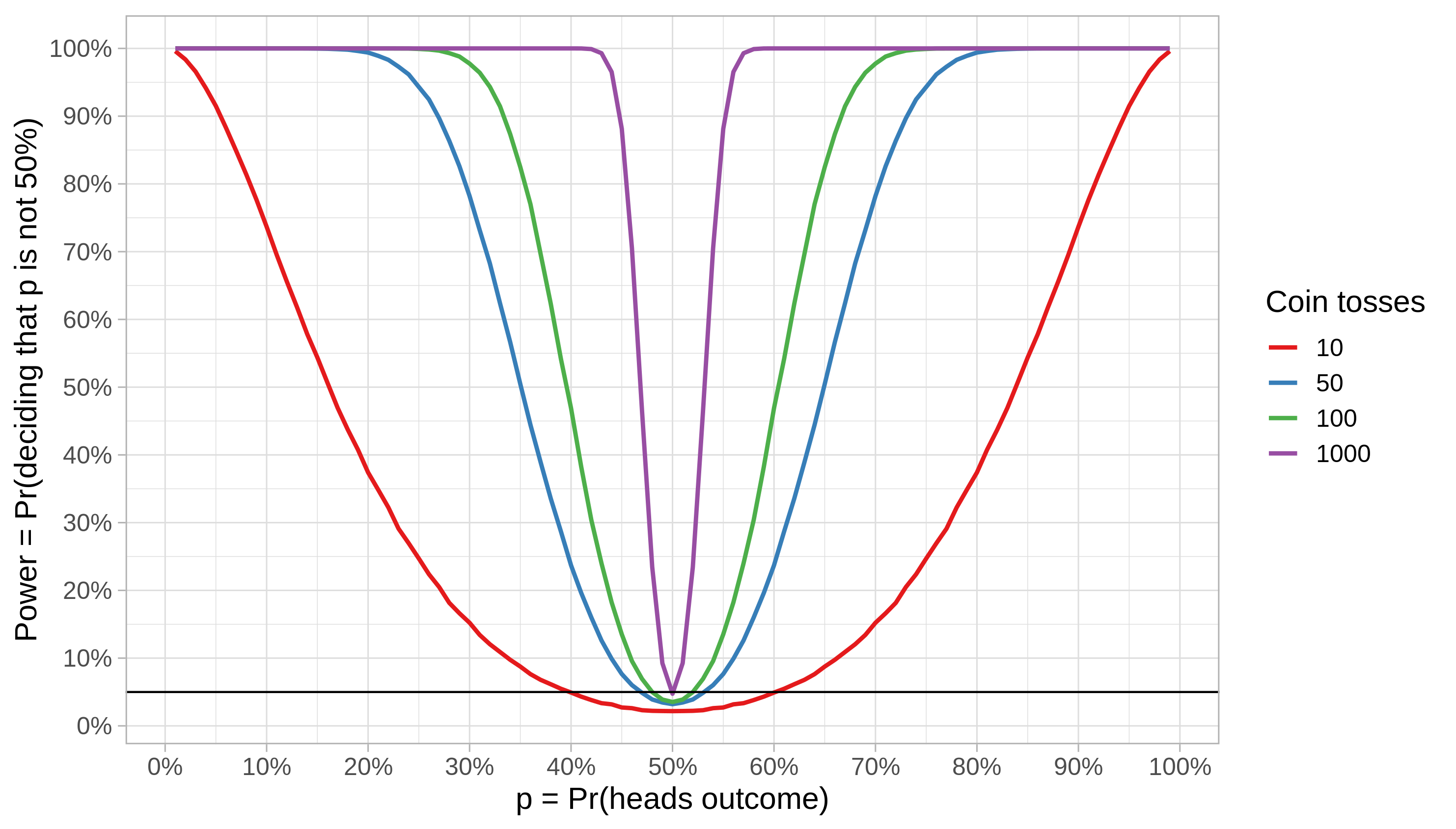
We can draw some conclusions from the power function above:
- The power grows as the true p gets more and more distant from the p induced by the null hypothesis (50%)
- Detecting deviations from the null hypothesis also becomes easier with more data from the same process. For instance, if the true p is between 40% and 60%, observing 100 instead of 10 coin flips lifts our rate of correct detections from 5% to 50%.
- The threshold distance from 50% for which the power reaches 100% is a function of the number of coin tosses. From the image, we see that this threshold is approximately 35% and 25% for 50 and 100 coin flips, respectively.
- The black line marks our pre-set, desired 5% FP rate. We see that our test procedure is sistematically conservative for small samples in the sense that the actual FP rate is always below the configured 5% rate; it gets closer to 5% as the number of coin tosses grows.
What is the reason for the conservative bias?
The probability of events as extreme as 2 heads in 10 coin tosses (that is, observing 0, 1, 2, 8, 9 or 10 heads) is 10.94%. We saw that this number is 2.15% for events as extreme as 1. The 5% FP rate we have pre-set is in-between these two numbers. The effect of the rule
Reject when p-value < 5%
under a discrete distribution is that our actual FP rate can be much smaller than 5%. That means less-than-specified, conservative FP rates.
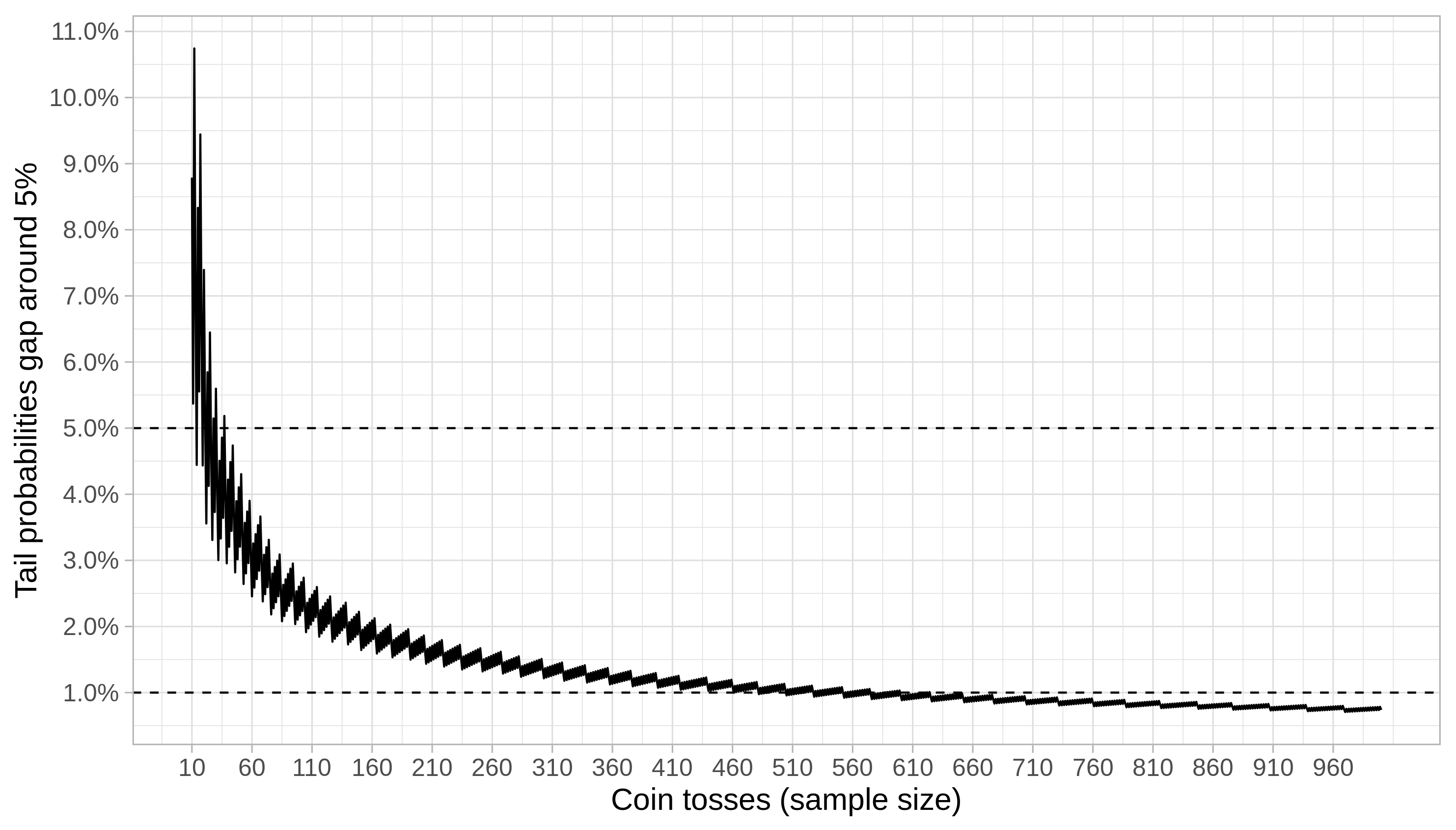
In our case, the sample size impacts the gap because it is an explicit parameter of the binomial distribution. The gap becomes negligible as the number of coin tosses grows, as we can see below. It remains consistently below 5% after the sample size becomes bigger than 37; that sample size threshold is 624 if we want to guarantee a gap less than 1%.
Can we do something about it?
We saw that by bounding the gap on tail probabilities of a binomial distribution we bound the conservative bias of our test. But, until now, for our case, the only solution is to increase the sample size. What if we can not gather more data? We want a test which always obeys the pre-set FP rate.
We can think about the FP rate as the expected value of a decision function. We’ve been using a function like that without realizing it because it’s trivial:
- Decision is 1 when p-value is less than 5%;
- Otherwise, decision is 0.
The (actual) FP rate is the expected value of this function:
\[\begin{equation} 1 \cdot P(\text{p_value} < 5\%) + 0 \cdot P(\text{p_value} \geq 5\%) = P(\text{p_value} < 5\%). \end{equation}\]Now, it’s easier to see the problem: \(P(\text{p_value} < 5\%)\) doesn’t necessarily yield 5% for discrete distributions as it was intended because of the gap problem we’ve discussed. In order to fix that, the idea is to randomize the decision function (w.p. is short for “with probability”):
- If p-value < 5%, decision is 1 w.p. \(\gamma\) and 0 w.p. \(1 - \gamma\);
- Otherwise, decision is 1 w.p. \(1 - \gamma\) and 0 w.p. \(\gamma\).
The constant \(\gamma\) is just a number chosen so that the actual FP rate, the expectation
\[\begin{equation} \gamma \cdot P(\text{p_value} < 5\%) + (1 - \gamma) \cdot \left[1 - P(\text{p_value} < 5\%)\right], \end{equation}\]equals the pre-specified FP rate, say \(\alpha\). Solving it for \(\gamma\):
\[\begin{equation} \gamma = \frac{1 - \alpha - P(\text{p_value} < 5\%)}{1 - 2 P(\text{p_value} < 5\%)}, \end{equation}\]In our case, for 10 coin tosses, the probability of hitting the threshold rule “p-value < 5%” is 2.15%, and it is related to observing 1 or 10 heads. Plugging that in the formula above, we obtain \(\gamma = 97.02\%\). Therefore, when we think we “saw something” (p-value < 5%), we only decide to reject the null hypothesis in 97.02% of the time. We “flip a coin” with probability \(\gamma\) to decide. Randomizing a decision may seen odd, but our expectation is that acting consistently according to this new rule, we will have better control over the FP rate.
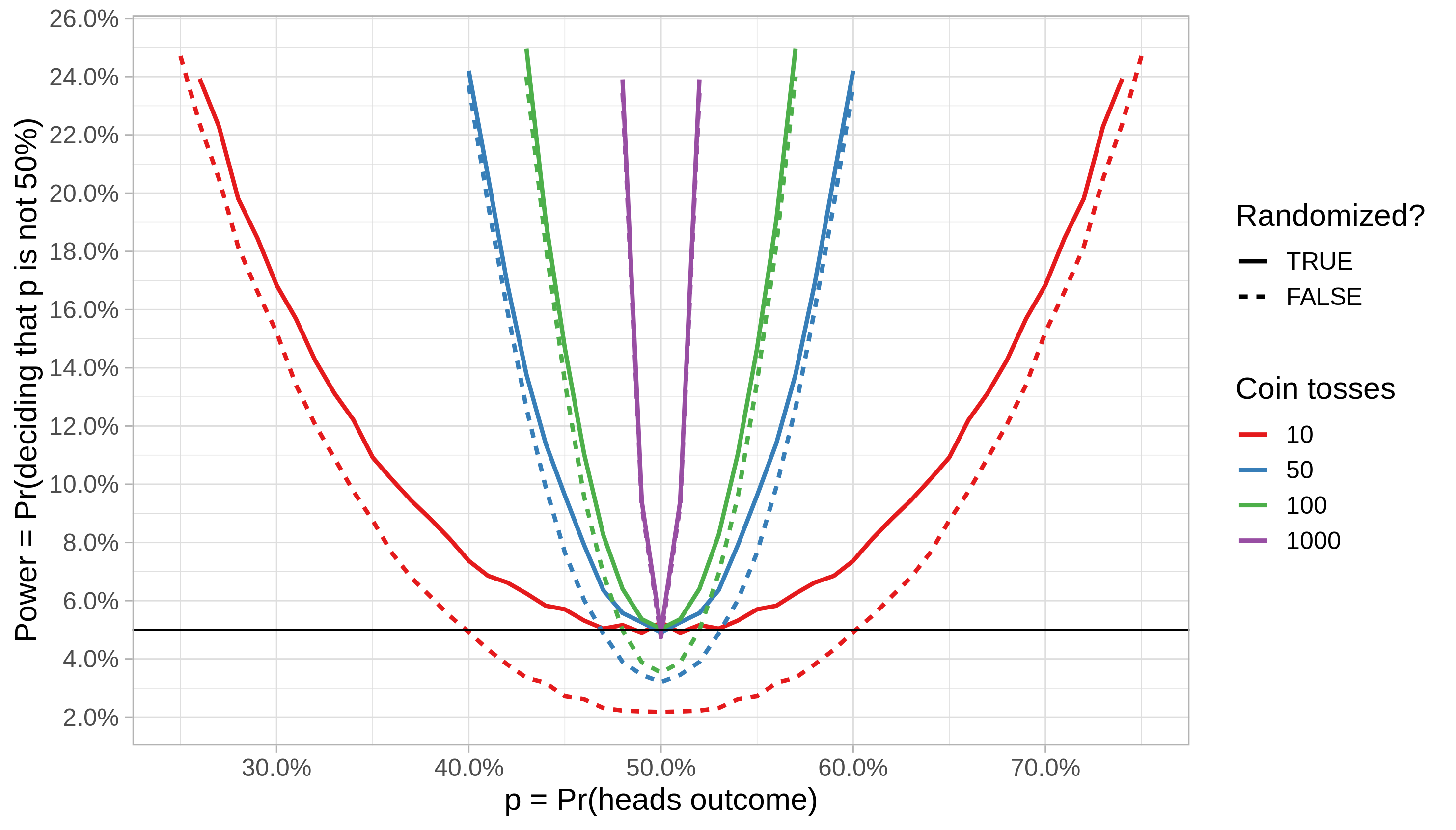
That is in fact what happens in the long run. Below is the power functions of both tests zoomed in the region around p = 1/2. We see that the actual FP rate now matches the pre-set FP rate in the randomized test, as intended, even for small sample sizes.
Do you trust it for your life?
Skin-in-the-game type of example
Real examples in more important situations are useful to realizing the relationship of the p-value to risk, and the importance of also having reliable estimates of power, besides accurate p-values.
Let’s say you want to do a surgery for changing your appearance. Not having the surgery does not kill you. It is just a “plus”. However, the doctor says that 1% of people die in the surgery table. Would you do it?
That answer can vary a lot amongst different people. The question of whether that 1% represents a reliable estimate of the probability of death for you in particular may be seen as too skeptical in trivial situations but probably we all agree that it’s reasonable here.
In common practical scenarios (e.g. health, finance, or business data analysis), we miss important properties which invalidate most naive, textbook analyses.
What is it for?
In our coin tossing example, we could come up with different models to make sense of the frequency of heads motivated by valid questions such as
- What if coin tosses are not independent from each other?
- What if our friend doesn’t tell the truth about the observed number of tails?
Answering that may look silly for coin tossing but similar skepticism is an important fuel to more serious research endeavors. That is a topic worth a post of its own.
Statistical machinery to model reality and then evaluate p-values accordingly can become as complicated as the problem asks for (or as skeptical you are). The rigor is proportional to how critical is to get it right, as with everything in life.
The important thing to have in mind is that
we don’t discover truths using these procedures, we identify lies.
If we have no evidence to reject the null hypothesis, we can’t be sure that it’s the ultimate truth, since that result can be explained by a multitude of hidden factors neither contained nor explained by the null hypothesis. But very small p-values in fact indicate that it’s very unlikely to support the (strong) claim made by the null hypothesis (“the world is like this”). Proving right is hard; detecting lies is easier.
Sum up
- The basic anatomy of a statistical test: hypothesis (model how the world may work), p-value evaluation (is it plausible to observe this in a world like that?), decide (or iterate);
- It’s impossible to get it right every time: the FPs versus FNs trade-off;
- Power estimates are as important as p-values in a way similar to confidence intervals being as important as point estimates;
- Different problems require different levels of rigor;
- Cultivating healthy skepticism may save your life.
Thanks for reading!