On selection bias and sample calibration
When using data from a sample of a population of interest to make inferences about that population, it’s important to be aware of the sampling process, i.e. how observed units in the sample were chosen.
The goals of this post are:
- To briefly introduce probability sampling;
- To talk about systematic selection biases and how we can reason about it;
- To expose the risk of being misled by selection bias when conclusions are driven by common statistical tools;
- Finally, to demonstrate what you can do about them and help you to understand the assumptions and consequent limitations of such tools.
This post is for anyone who is interested on these issues and has a basic understanding of probability and statistics.
I’ll discuss these topics in a simple yet realistic setup. I’ll take advantage of the simplicity to make a deeper analysis that’s hopefully useful in understanding the technique as applied in the wild.
The problem
We are interested in a finite population, or universe, \(U = \{1,2,\ldots,N\}\) of \(N\) elements, or units, and only a sample \(S \subset U\) of \(n\) elements taken from \(U\) is available. We want to use \(S\) to provide a guess, or estimate, for the populational quantity, or parameter,
\[\begin{equation} P(C) = \frac{N(C)}{N}, \end{equation}\]the proportion of elements of \(U\) that belong to a set \(C \subset U\). We write \(N(X)\) and \(n(X)\) for the number of elements of \(X\) in \(U\) and \(S\), respectively. You can also think of \(P(C)\) as the probability of sampling a random element from \(U\) and then finding out that it belongs to \(C\). These two interpretations (the “share of something” in the population and the “probability of something” being sampled) can be invoked interchangeably througout the text whenever you see \(P(\text{something})\). Also, recall the definition of conditional distributions:
\[P(X \mid Y) = \frac{P(X \cap Y)}{P(Y)},\]where \(X\) and \(Y \neq \emptyset\) are subsets of \(U\).
The population in one figure
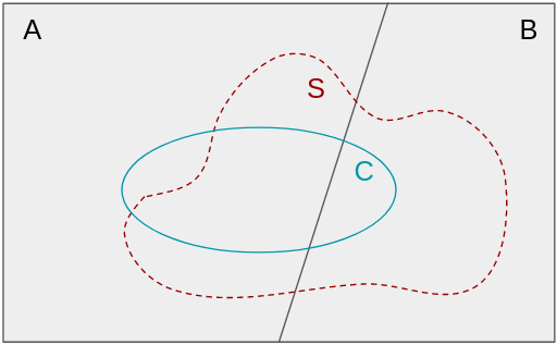
That situation can be visualized below, where the whole rectangle is \(U\) and we also add that it can be partitioned into two disjoint sets \(A\) and \(B = A^c\) (just the complement of \(A\) in \(U\)), which are going to be useful in a minute.
You can think of \(A\) as being any other characteristic of the elements of \(U\) that may be important to understand those which belong to \(C\). Both \(A\) and \(C\) could be some thresholding on age, years of education or gender in case we are talking about humans.
Probability sampling
We say that \(S\) is a probability sample if it was obtained by a controlled (i.e. known) randomization procedure that attaches to each element \(i \in U\) an inclusion probability \(\pi_i\) of it being chosen to be part of \(S\).
For a set \(X \subset U\), we define the binary variable \(X_i\) as being 1 when \(i \in X\) and 0 otherwise.
Note that \(C_i\) is just a constant that can be perfectly known as long as we have access to the unit \(i\). On the other hand, we only get to know the \(S_i\) values once we get \(S\), and repeating the same randomized sampling process may yield different values for the same \(i\). If the sampling procedure itself is known, then what we know a priori is the inclusion probability \(P(S_i = 1) = 1 - P(S_i = 0) = \pi_i\). That is, prior to sampling, \(S_i\) is a Bernoulli random variable.
Now we may write
\[P(C) = \frac{N(C)}{N} = \frac{1}{N} \sum_{i \in U} C_i.\]Let’s try to employ the sample analogue of the above equation to estimate \(P(C)\) from \(S\) (just because it is pretty intuitive):
\[\widehat{P(C)} = \frac{1}{n} \sum_{i \in S} C_i.\]Note that \(\widehat{P(C)}\) is a random variable because it depends on \(S\), which prior to sampling we do not know. Let’s make the dependence on the random process explicit in terms of the \(S_i\) variables (note the change from \(S\) to \(U\) in the second summation):
\[\widehat{P(C)} = \frac{1}{n} \sum_{i \in S} C_i = \frac{1}{n} \sum_{i \in U} C_i \cdot S_i.\]Is this an accurate estimator of \(P(C)\)? Since the \(C_i\)s are constants, it’s easy to compute the expectation of this random variable:
\[\begin{align} \mathrm{E} \left\{ \widehat{P(C)} \right\} &= \mathrm{E} \left\{ \frac{1}{n} \sum_{i \in U} C_i \cdot S_i \right\} \\ &= \frac{1}{n} \sum_{i \in U} C_i \cdot \mathrm{E} \left\{ S_i \right\} \\ &= \frac{1}{n} \sum_{i \in U} C_i \cdot \pi_i. \end{align}\]When all units \(i\) are equally likely to be sampled, we have that \(\pi_i = n/N\) for all \(i\). In this case, \(S\) is called a simple random sample (SRS) and the equation collapses into
\[\begin{align} \mathrm{E} \left\{ \widehat{P(C)} \right\} = \frac{1}{N} \sum_{i \in U} C_i = P(C). \end{align}\]That is, under a SRS, the sample proportion of cases in \(C\) is a nice guess of its populational counterpart. When an equation like this holds true, we say that the estimator is centered for the parameter.
The Horvitz-Thompson estimator
But what if \(S\) is not a SRS? What if the elements in \(U\) are not equally likely to be in \(S\)?
An important observation is that both \(P(C)\) and \(\widehat{P(C)}\) are linear combinations of the \(C_i\)s. Let’s write it down:
\[\widehat{P(C)} = \sum_{i \in S} k_i \cdot C_i,\]where the \(k_i\)s are constants. In the SRS case, we just saw that \(k_i = 1/n\) is a good choice because \(\pi_i = n/N\). In general, we observe that the expectation of this linear estimator is
\[\begin{align} \mathrm{E} \left\{ \widehat{P(C)} \right\} &= \mathrm{E} \left\{ \sum_{i \in U} k_i \cdot C_i \cdot S_i \right\} \\ &= \sum_{i \in U} k_i \cdot C_i \cdot \pi_i. \end{align}\]If we set \(k_i = (N \pi_i)^{-1}\), then \(\widehat{P(C)}\) is centered for \(P(C)\). This is known as the Horvitz-Thompson estimator (HTE). It assumes that we know the randomization process that yields \(S\) and therefore know the inclusion probabilities \(\pi_i\) up to reasonable accuracy for all \(i\).
Notice that probability sampling designs may have different inclusion probabilities for different units in the population (SRS is not the only probability sampling design). That is simply a design choice that is commonly employed as a tool to improve the precision of the estimates under certain circumstances.
But what if we do not know the \(\pi_i\)s? Equivalently, what if we do not know the process that yields \(S\)? Well, welcome to most real-world data analysis problems.
Calibration
In practice, we rarely know the structure of the sampling process. However, when we do know it, we saw that the HTE proposes to weight the data from unit \(i\) with \((N\pi_i)^{-1}\) and this choice produces a centered estimator. That’s nicely intuitive since we may interpret \(\pi_i^{-1}\) as the number of units in \(U\) that the unit \(i\) will be responsible to represent in case it’s sampled.
The baseline approach is usually the sample proportion, which we know to be our best guess of \(P(C)\) under SRS. How can we improve it?
Let’s suppose that knowing that an unit belongs to \(A\) is a relevant piece of information to guess whether or not it is also in \(C\). In other words, \(A\) and \(C\) are correlated and then the distribution \(P(C \mid A)\) is different from \(P(C)\). We’ll denote this hypothesis by \(\mathcal{H}\).
From the law of total probability, we have
\[\begin{align} P(C) = P(C \mid A) \ P(A) + P(C \mid B) \ P(B). \end{align}\]A similar equation is also true when we condition on the sample as well:
\[\begin{align} P(C \mid S) &= P(C \mid A \cap S)\ P(A \mid S) + P(C \mid B \cap S) \ P(B \mid S). \end{align}\]It may be useful to visualize these equations in the figure at the beginning. Note that \(P(C \mid S)\) is just the baseline estimate, the fraction of \(C\) in \(S\) once \(S\) is realized. Also, it’s informative to evaluate this last equation for the SRS case, just to convince ourselves that it makes sense:
\[\widehat{P_{\text{SRS}}(C)} = \frac{n(C \cap A)}{n(A)} \frac{n(A)}{n} + \frac{n(C \cap B)}{n(B)} \frac{n(B)}{n} = \frac{n(C)}{n},\]which is right! We’ve used the fact that \(A\) and \(B\) form a partition of \(U\) and we removed the conditioning on \(S\) and now we have a random variable.
What I want to point out now is how we may improve this estimator induced by \(P(C \mid S)\) given that we do not know the structure of the sampling process but \(\mathcal{H}\) is true and we have access to auxiliary information on \(P(A)\) in the form of an alternative estimate \(\widehat{P(A)}\).
The (observed) bias of our baseline estimator is \(P(C \mid S) - P(C)\). Hopefully, it’s clear that it has two sources:
- \(P(A \mid S) \neq P(A)\): Under \(\mathcal{H}\), over- or under-representation of \(A\) in \(S\) can be a problem since we want to estimate \(P(C)\);
- \(P(C \mid A \cap S) \neq P(C \mid A)\) (similarly for \(B\)): Even when the previous point is OK, we can still suffer if there is selection bias within \(A\) and \(B\) with respect to \(C\).
It’s a good exercise to verify that both inequalities above turn into equalities under SRS. It’s also important to notice that these can cause problems when we use the baseline fraction-of-\(C\)-in-\(S\) estimator and these issues are present. In general, these conditions can be met by probability sampling designs and that would not be a problem because we would be aware of it and could employ, say, the HTE. We want to analyze the disparities between a naive guess and possible underlying populational realities.
The idea is simply to substitute \(P(A \mid S)\) by the auxiliary estimate \(\widehat{P(A)}\), with \(\widehat{P(B)} = 1 - \widehat{P(A)}\), to obtain
\[\begin{align} \widehat{P_\text{calib}(C)} &= \widehat{P(A)} \frac{n(C \cap A)}{n(A)} + \widehat{P(B)} \frac{n(C \cap B)}{n(B)} \\ &= \sum_{i \in S} \left( \frac{\widehat{P(A)} \cdot A_i \cdot C_i}{n(A)} + \frac{\widehat{P(B)} \cdot B_i \cdot C_i}{n(B)} \right). \end{align}\]This technique is known as calibration. As discussed, it’s expected to work as fine as the sample approximations of the conditional distributions \(P(C \mid A)\) and \(P(C \mid B)\).
This estimator is also linear in \(C_i\) and the HTE coefficient \(k_i = (N\pi_i)^{-1}\) is being estimated as \(\widehat{P(A)}/{n(A)}\) if \(i \in A\), and \(\widehat{P(B)}/{n(B)}\) otherwise. Also, whenever \(\widehat{P(A)}\) is a good approximation, i.e. \(\widehat{P(A)} \approx P(A) = N(A)/N\), we get
\[\frac{\widehat{P(A)}}{n(A)} = \left( N \cdot \frac{n(A)}{N(A)} \right)^{-1},\]and thus we are estimating the inclusion probability \(\pi_i\) as the probability \(n(A)/N(A)\) that a random unit from \(A\) will be found to be in \(S\) (take a second to think about it).
That’s how our assumptions plus this calibration thing are effectively modeling the sampling process.
It seems reasonable to argue that if we have no prior information on the \(\pi_i\)s, our expectation on the statistical performance of \(\widehat{P_\text{calib}(C)}\) is always equal to or better than that of \(\widehat{P_\text{SRS}(C)}\) whenever \(\widehat{P(A)}\) is more accurate than \(n(A)/n\).
Sum up
We’ve learned that
- Under SRS, the commonly used sample proportion is a good guess for the populational proportion
- When that is not the case but we know the sampling process, the general form of the proportion estimator is given by the Horvitz-Thompson estimator, in which each unit \(i\) is assigned a weight proportional to \(\pi_i^{-1}\);
- When we do not know the sampling process but we have access to information on auxiliary variables that correlate with the variable we want to understand, we can use this extra info to calibrate our naive sample proportion and expect its performance to improve a bit, depending on how strong is that correlation.
In a future post, I hope to show the technique in action with real data.
Thanks for reading.